Exploring classifiers and cross-validation techniques for Digits and Iris datasets
We are presently interested in solving some relatively simple machine learning problems - digit recognizer and Iris. The size of these datasets is somewhat small, so we will explore some options to get the best accuracies for our model.
The data
We are working on two sets of data: the digits dataset and the Iris dataset. We will import these datasets directly from the scikit-learn standard datasets.
from sklearn import datasets
iris = datasets.load_iris()
digits = datasets.load_digits()
These datasets are provided in dictionary-like objects. The digits dataset has 1797 samples and the Iris dataset has 150 samples. As mentioned earlier, these are particularly small datasets, which poses an additional challenge to train our models. We can take a peek at these two datasets:
print(iris.data,iris.target)
[[5.1 3.5 1.4 0.2] [4.9 3. 1.4 0.2] [4.7 3.2 1.3 0.2]
….. [4.6 3.1 1.5 0.2] [5. 3.6 1.4 0.2] [5.4 3.9 1.7 0.4]
[0 0 0 0… 1 1 1 1 1 1 2 2 2]
print(digits.data,digits.target)
[[ 0. 0. 5. … 0. 0. 0.] [ 0. 0. 0. … 10. 0. 0.] [ 0. 0. 0. … 16. 9. 0.] … [ 0. 0. 1. … 6. 0. 0.] [ 0. 0. 2. … 12. 0. 0.] [ 0. 0. 10. … 12. 1. 0.]] [0 1 2 … 8 9 8]
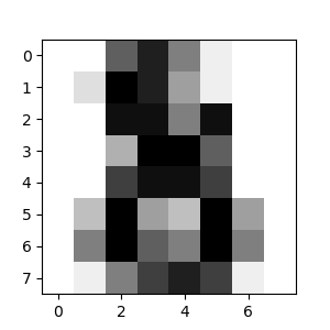
The Iris dataset has 4 attributes (corresponding to the flower; see details here) and the Digits dataset has 64 attributes (8x8 pixel values) as shown below.
Our task here is to train a machine learning model with this small dataset and cross-validate the model to quantify the accuracy of the model.
Classifiers
The choice of the classifier is, in general, not known a priori, although some classifier algorithms are better suited for certain types of problems (for instance, Naive Bayes is well-suited for spam detection). We will presently explore some classifier algorithms that would be best suited for our purposes. Before that, we will do some basic data preprocessing:
from sklearn.preprocessing import StandardScaler
X = digits.data
X = StandardScaler().fit_transform(X)
y = digits.target
SVM
SVM (Support Vector Machines) algorithm is quite well-suited for multi-class classification problems, and they are effective for higher dimensional feature data. The ability to use different Kernel functions means that this algorithm can be applied to different kinds of data. The implementation is as follows:
from sklearn import svm
clf = svm.SVC(gamma=0.001, C=100., kernel = 'rbf')
Tuning parameters
The important parameters to tune in this algorithm are the kernel function, gamma and C values. A linear kernel function is good enough when the boundaries between the classes are simple and well-defined. For our case, RBF kernel function can be expected to give the best results since the boundaries between classes are rather complex.
K nearest neighbors
The choice of using KNN algorithm for our problem is a natural one. This is a non-parametric method that can be used for both classification and regression. Features are grouped based on their vicinity to other features. This also happens to be a rather simple algorithm to implement with relatively few parameters to tune. The implementation is as follows:
from sklearn.neighbors import KNeighborsClassifier
clf = KNeighborsClassifier(4)
Tuning parameters
The most important parameter to tune is the choice of K. Larger the value of K, smaller the effect of noise. Smaller values of K makes the distinction between the classes rigid, and hence is more sensitive to noise. We can quickly check the effect of varying K with a plot as shown below:
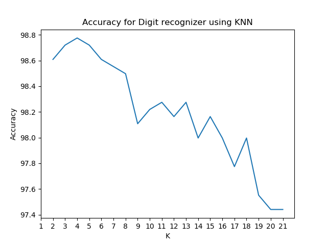
Based on this above plot, we choose the value of K = 4.
Multi-layer Perceptron classifier
MLP classifier is a feed-forward neural network algorithm. From Wikipedia: A MLP consists of at least three layers of nodes: an input layer, a hidden layer and an output layer. Except for the input nodes, each node is a neuron that uses a nonlinear activation function.
The implementation is as follows:
from sklearn.neural_network import MLPClassifier
clf =  MLPClassifier(alpha=1,solver='lbfgs')
Tuning parameters
The solver for this algorithm is typically chosen as ‘adam’, but given the small size of our dataset, it is much more effective and efficient to use ‘lbfgs’. We will use the default ‘relu’ activation function, and an alpha value = 1.
Cross-validation
LeaveOneOut versus K-fold: When dealing with a small dataset like here, it is important to use a cross-validation technique to ensure that we are not overfitting. A rudimentary method for cross-validation is the LeaveOneOut technique. Here, the dataset is split into train/validation splits in the ratio n-1:1. In other words, the model is trained using n-1 samples and tested on the n_th sample. This is repeated _n times and the accuracy obtained is the average of them all. While this algorithm tends to give the best accuracy, it can be computationally very intensive.
To overcome this, we can use a more general technique for cross-validation called the KFold cross validation technique. Here, the data is divided into k consecutive folds; each fold is once used to train the model and the k-1 folds form the training set. The value of k is in the user’s control and can be varied. In general, larger values of k give higher accuracies. We will study the effect of the value of k in determining prediction accuracy for two values of k: k = 10 and k = 50.
Note that the LeaveOneOut algorithm is equivalent to using KFold with k = number of samples.
Summary
We can summarize all the results obtained above in the following table:
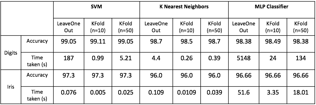
We see that SVM is a good algorithm for our purposes as it provides a nice tradeoff between performance and time taken. In this dataset, it is not necessary to use the expensive LeaveOneOut validation technique and we can instead make do with KFold with n=10.
The code to generate these results can be obtained here.