Exploring performance metrics of classification algorithms

In this post, we will explore the various performance metrics for classification algorithms. We will use a popular dataset to predict income class (whether a person of the population makes more than 50K or not). The dataset is available on UCI Machine Learning database: https://archive.ics.uci.edu/ml/datasets/census+income.

The prediction task involves the following standard steps:

1. loading the training data,
2. conduct exploratory data analysis,
3. conduct some preprocessing and cleaning,
4. fit classification models to training data,
5. make predictions on the test data,
6. the performance of the models using metrics.

We will start by first loading the important modules and the training dataset. Pandas and scikit-learn are the important modules we will be using here.

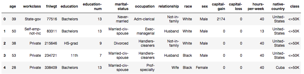
Our input data consists of both categorical and numeric features. The last column is the dependent variable. We have to do a few things now - separate the raw data into independent features and dependent feature (label), identify if any features are double counted or are irrelevant, then encode the categorical features and the output label.

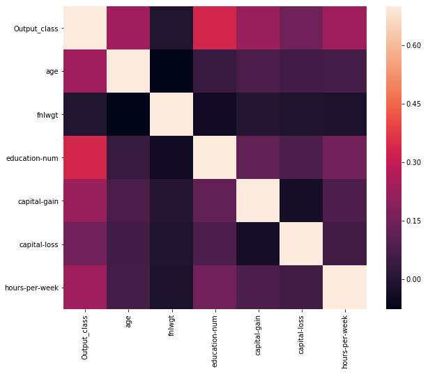
We see that the feature fnlwgt is not correlated at all with the output class, so we can safely drop that feature. Also, we see that there are two features describing eduction level - “education” and “education_num”. So, we can drop the categorical feature “education”.

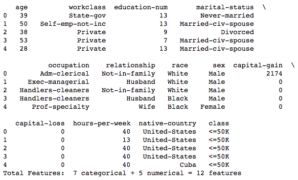
We note that we have both categorical features and numerical features. The categorical features are encoded using OneHotEncoder, which is the standard encoder used for non-cardinal features.

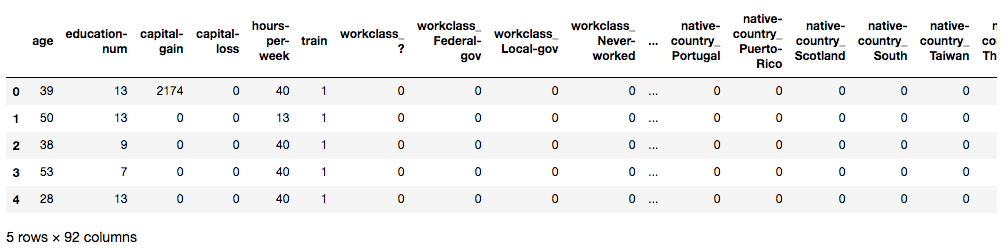
We would ideally like to use OneHotEncoder to encode the categorical features (since none of them have any cardinality). But, in one of the features, there are more distinct values in the training data than in the test data. So, if we apply OneHotEncoder to the two datasets separately, there is one more column in the training data than in the test data. One way to overcome this is to combine the two datasets, apply the encoder on the combined dataset, and then separate the training and test datasets, as below:

Shown below is a snippet of the output:

We’re almost ready to train models with the dataset. One last step is to normalize/scale the features such that they are of comparable magnitudes. We will use StandardScaler for this purpose. Further, we will apply a series of standard classification algorithms.

Now, we have fit the training data to many classification algorithms with some standard parameters, and calculated probabilities. We will use these for evaluating the models.

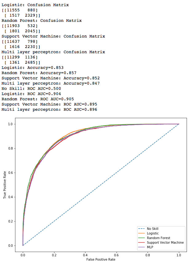
In summary, we have used four different machine learning algorithms to make predictions about the income class. All four classification models give reasonable accuracies, with Random Forest algorithm providing the best accuracy. We also used area under the ROC curve as a metric and we saw that Random Forest performs best again. We can definitely perform much better on these models with some parameter tuning, which we will undertake in an upcoming post.