Artificial Neural Network to predict housing prices - Part 1
This project involved the use of the popular Ames Housing dataset: http://jse.amstat.org/v19n3/decock.pdf. The dataset contains 2930 observations and a large number (80) of explanatory variables (23 nominal, 23 ordinal, 14 discrete, and 20 continuous) involved in assessing home values. The dataset is divided into training and test datasets and an artificial neural network (ANN) is implemented to predict the housing prices of the test dataset. For this, Keras/Tensorflow libraries are used to train the model and predict. An exploration of several parameters of the model such as the activation function, bias function and number of layers in the neural network was undertaken to identify the best parameters for this problem. K-fold cross-validation is used to examine the effectiveness of the model. Finally, a grid-search algorithm is used to perform hyperparameter optimization to ensure that we find the best parameters. In the first part, we will only explore the dataset, build a model and predict prices. The evaluation of the model and its improvement will be reserved for another post.
Okay, so we start with importing the relevant Python modules. We will use Pandas for to work with the data and Keras to build the neural network.
import numpy as np
import matplotlib.pyplot as plt
import pandas as pd
import keras
from keras.models import Sequential
from keras.layers import Dense
Now, we will import the data from the csv file using Pandas:
dataset = pd.read_csv("all/train.csv")
dataset.iloc[:,3] = dataset.iloc[:,3].fillna(0)
As mentioned above, this dataset has a huge number of features (80). Let us first take a look at the column names and then use our judgment to decide the most important features. Instead of blindly feeding every feature to the algorithm, it is better to do some manual screening at this point.
dataset.head(0)
Columns: [Id, MSSubClass, MSZoning, LotFrontage, LotArea, Street, Alley, LotShape, LandContour, Utilities, LotConfig, LandSlope, Neighborhood, Condition1, Condition2, BldgType, HouseStyle, OverallQual, OverallCond, YearBuilt, YearRemodAdd, RoofStyle, RoofMatl, Exterior1st, Exterior2nd, MasVnrType, MasVnrArea, ExterQual, ExterCond, Foundation, BsmtQual, BsmtCond, BsmtExposure, BsmtFinType1, BsmtFinSF1, BsmtFinType2, BsmtFinSF2, BsmtUnfSF, TotalBsmtSF, Heating, HeatingQC, CentralAir, Electrical, 1stFlrSF, 2ndFlrSF, LowQualFinSF, GrLivArea, BsmtFullBath, BsmtHalfBath, FullBath, HalfBath, BedroomAbvGr, KitchenAbvGr, KitchenQual, TotRmsAbvGrd, Functional, Fireplaces, FireplaceQu, GarageType, GarageYrBlt, GarageFinish, GarageCars, GarageArea, GarageQual, GarageCond, PavedDrive, WoodDeckSF, OpenPorchSF, EnclosedPorch, 3SsnPorch, ScreenPorch, PoolArea, PoolQC, Fence, MiscFeature, MiscVal, MoSold, YrSold, SaleType, SaleCondition, SalePrice]
It is a good idea here to visualize the role of the individual features in determining the housing prices. Some obvious contenders to look into initially are LotArea (Area of the lot), OverallQual (Overall quality), YearBuilt (Year built), TotRmsAbvGrd (Total rooms above ground) and GarageArea. We will plot each of these features against SalePrice (Sale price) to check the role of these features.
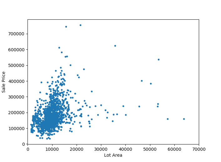
As expected, there is a weak linear correlation between the lot area and the sale price.
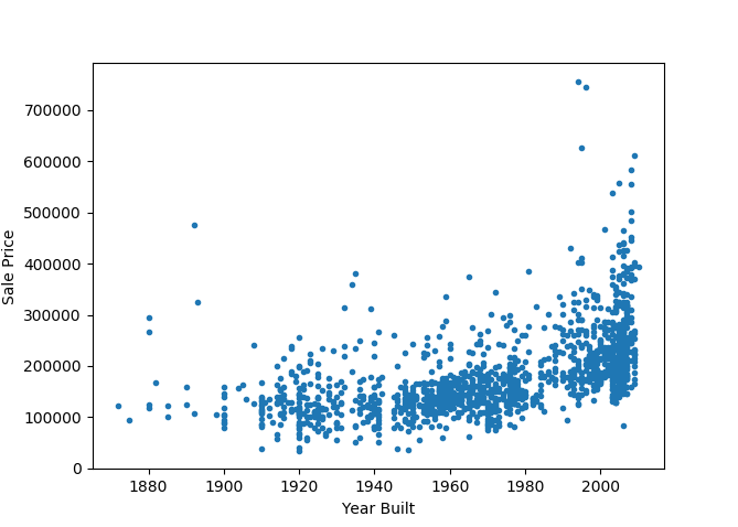
Now, this is surprising as I had expected the year built to have a more significant role in determining housing prices. But anyway, it clearly plays a marginal role and it makes sense to include this feature in the overall analysis.
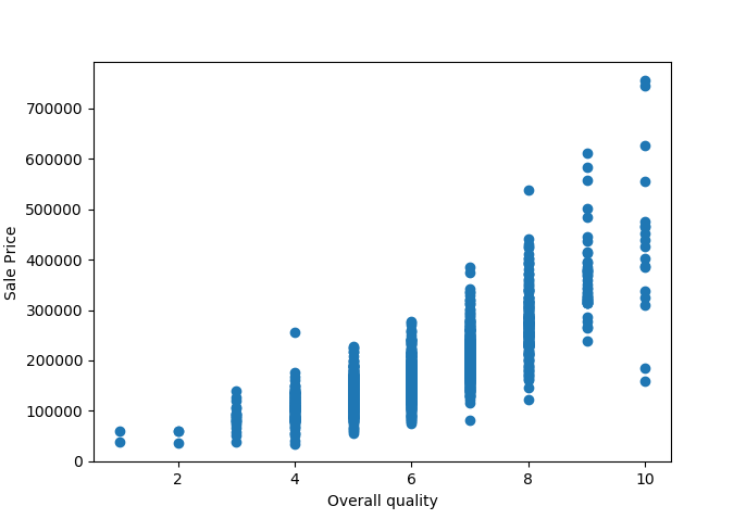
The Overall Quality metric plays a significant role and it’s a no-brainer that we need to include this feature in the analysis.
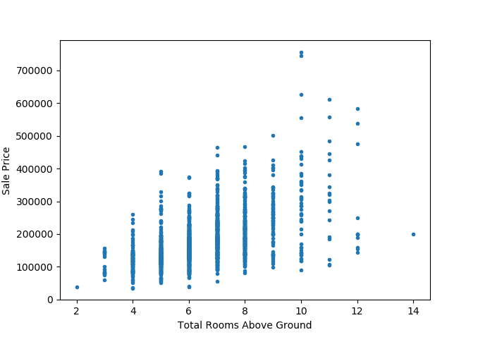
The total number of rooms in the house seems to have an almost normal distribution. But then again, we have a rather limited number of data points at the larger end of the spectrum (of number of rooms). Nevertheless, it is evident that this metric plays an important role in contributing to the sale price.
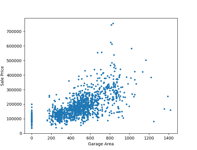
One could argue at this point that the garage area is an indirect measure of the lot area. To ensure we are not double-counting the lot area, we will take a quick look at the relationship between the two features.
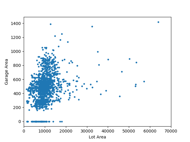
Okay, while there is some weak correlation, there is sufficient spread between the two variables to consider both the features. In addition to these features, we include several other features based on their relevance to the sale price into the model. These are shown below. It’s a good practice to examine the role of individual features on the feature label (of the training dataset), especially when we have such a large number of features. So, off to building the regression model.
X = dataset.iloc[:, [1,2,3,4,12,17,19,46,27,53,54,56,79,43,44,62]].values
y = dataset.iloc[:, 80].values
y = np.reshape(y, (-1,1))

dataset.iloc[:,1] = dataset.iloc[:,1].fillna(0)
Now, among the features that we have selected, a number of them are categorical variables. For instance, MSZoning, which identifies the general zoning classification of the sale (such as Agricultural, Industrial, Commercial etc) is a categorical variable. We need to encode these categorical variable, i.e., assign integer labels to them before we fit the model.
from sklearn.preprocessing import LabelEncoder, OneHotEncoder
labelencoder_X_1 = LabelEncoder()
X[:, 1] = labelencoder_X_1.fit_transform(X[:, 1])
labelencoder_X_4 = LabelEncoder()
X[:, 4] = labelencoder_X_4.fit_transform(X[:, 4])
labelencoder_X_8 = LabelEncoder()
X[:, 8] = labelencoder_X_8.fit_transform(X[:, 8])
labelencoder_X_9 = LabelEncoder()
X[:, 9] = labelencoder_X_9.fit_transform(X[:, 9])
labelencoder_X_12 = LabelEncoder()
X[:, 12] = labelencoder_X_12.fit_transform(X[:, 12])
Another element of preprocessing of the feature data before feeding into the model involves feature scaling. Feature scaling is performed to ensure that the ranges of the features are not varying wildly.
from sklearn.preprocessing import MinMaxScaler
sc = MinMaxScaler()
print(sc.fit(X))
X_train = sc.transform(X)
Now, we are in a position to build the neural network.
model = Sequential()
model.add(Dense(12, input_dim=16, kernel_initializer='uniform', activation='relu'))
model.add(Dense(6, kernel_initializer='uniform', activation='relu'))
model.add(Dense(1, kernel_initializer='uniform', activation='relu'))
model.summary()
model.compile(loss='mse', optimizer='adam', metrics=['mse','mae','accuracy'])
There is a lot to unpack in these above lines. We are first defining a Sequential neural network. We then add Dense layers to the network. The activation function used here is relu which is a robust function. We add an intermediate layer (after the initial layer) and the output layer. The number of dimensions in the initial and middle layer is determined after testing to optimize for better performance, and this is done using the guideline of having the middle layer as approximately half the sum of the input and output layers. The last line compiles the model and the loss function is defined as the mean squared error, and we use the adam optimizer.
Now we will go ahead and fit the model to the training dataset and visualize the evolution of the loss function with the number of epochs.
history = model.fit(X_train, y, epochs=1000, batch_size=20,  verbose=2,validation_split=0.2)
plt.plot(history.history['loss'])
plt.title('model loss')
plt.ylabel('loss')
plt.xlabel('epoch')
plt.legend(['train', 'validation'], loc='upper left')
plt.show()
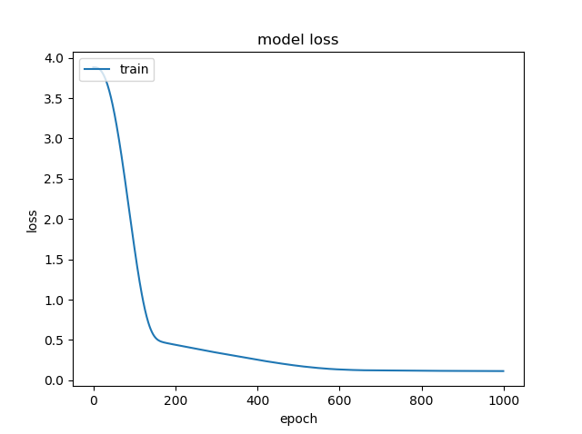
It’s good to note that the loss function is decreasing with the number of epochs. This seems to saturate at around 600 epochs. Now, we will read in the test dataset and predict the prices for that. We will perform the same preprocessing steps on the features as we did for the training dataset, namely encoding categorical variables and feature scaling.
dataset_test = pd.read_csv("all/test.csv")
dataset_test.iloc[:,53] = dataset_test.iloc[:,53].fillna("UNKNOWN")
dataset_test.iloc[:,62] = dataset_test.iloc[:,62].fillna(0)
dataset_test.iloc[:,3] = dataset_test.iloc[:,3].fillna(0)
X_test = dataset_test.iloc[:, [1,2,3,4,12,17,19,46,27,53,54,56,79,43,44,62]].values

# Encoding categorical variable
from sklearn.preprocessing import LabelEncoder, OneHotEncoder
labelencoder_X_test_1 = LabelEncoder()
X_test[:, 1] = labelencoder_X_test_1.fit_transform(X_test[:, 1].astype(str))
labelencoder_X_test_4 = LabelEncoder()
X_test[:, 4] = labelencoder_X_test_4.fit_transform(X_test[:, 4])
labelencoder_X_test_8 = LabelEncoder()
X_test[:, 8] = labelencoder_X_test_8.fit_transform(X_test[:, 8])
labelencoder_X_test_9 = LabelEncoder()
X_test[:, 9] = labelencoder_X_test_9.fit_transform(X_test[:, 9])
labelencoder_X_test_12 = LabelEncoder()
X_test[:, 12] = labelencoder_X_test_12.fit_transform(X_test[:, 12])

X_test = X_test.astype(np.float)

# Feature Scaling
from sklearn.preprocessing import MinMaxScaler
sc2 = MinMaxScaler()
X_testscaled = sc2.transform(X_test)
We are finally ready to predict the housing prices for the test dataset.
y_pred=model.predict(X_testscaled)
That is it- we have a first approximation on the predicted housing prices. Of course there is plenty of work to be done before we are happy with the results. K-fold cross-validation to evaluate the model and then parameter tuning to improve the model are all necessary next steps. But that will be undertaken in an upcoming post.