Sampling, resampling and hypothesis testing
Continuing on the list of posts on statistics and quantitative analysis, this is a compilation of some routines for statistical analyses in Python. This work will be done using scipy.stats and numpy libraries. These codes are inspired by Allen Downey’s Think Stats book and lectures.
Typically, in real life statistical applications, we do not have access to the dataset from the entire population. Instead, what we have is a small subset of the population, also called a sample.
Drawing samples from a normal distribution
We will first create an arbitrary normal distribution. This distribution is a representation of the male heights in the United States.
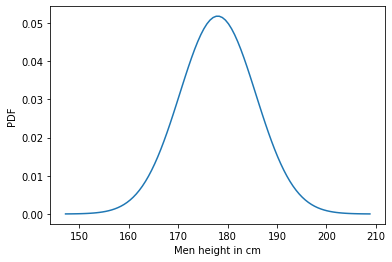
Now, we would like to draw/sample some values from the distribution.
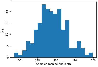
As long as our sample size is large enough, the sampled distribution resembles that of the original population distribution.
Resampling methods - Bootstrapping
We had the convenience of having access to the actual distribution of the data and its mean, standard deviation. This data was sourced from a large database of heights of US men (~300000 samples).
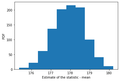
But typically, we do not have access to the distribution. Estimates of central tendency (mean) and dispersion (standard deviation) in those cases are not readily available. In such cases when we just have a reasonably sized dataset (let’s say 1000 data points), we have to resort to resampling methods, the most common one being Bootstrapping. In bootstrapping, we resample from the same dataset WITH REPLACEMENT and compute our estimates. Thanks to Central Limit Theorem (CLT), we end up with a normal distribution of the estimate (as long as we sample enough times). CLT states that when independent random variables are added, their normalized sum tends toward a normal distribution. The place where CLT shines is that the initial distribution does not have to be normal for the estimates to be normally distributed. In fact, we don’t even need to know the type of distribution of the original dataset. But, typically, the farther away from a normal distribution the data is (think pareto distribution), more times we have to resample.
We will first obtain an estimate for mean and std for the normally distributed data, then for a random distribution.
The plan is to take a sample from the population (akin to what we would have in real life) and estimate some sample statistics using Bootstrapping.
Estimated statistic = 177.937
Standard error = 0.798
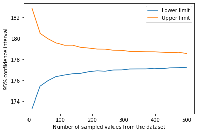
95% confidence interval = [176.33743211 179.39532095]
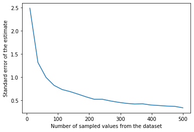
As expected, the standard error should decrease with increase in the number of sampled data. But it is pretty much immune to the number of iterations. Also, evidently, the confidence interval shrinks in size as we increase the size of the sampled data.
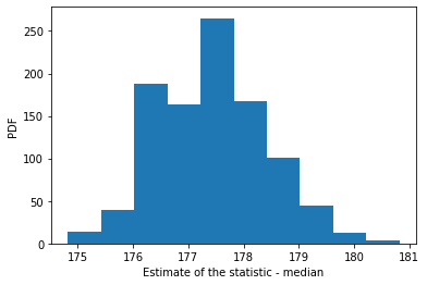
The remarkable thing about CLT is that the above method can be used to estimate any quantity, not just the mean. Median, standard deviation, coefficient of determination, you name it. This procedure simply involves changing the calculated statistic above. We will repeat the process for estimating the median.
Estimated statistic = 177.437
Standard error = 0.973
95% confidence interval = [175.68731829 179.51358241]
Some comments
It is important to understand what the confidence interval actually represents.
What the confidence level DOES NOT represent: The confidence level is not a suggestion about whether the estimated parameter lies within the interval or not. The confidence interval provides no indication about whether the estimate lies within the limit or not. Whether or not the estimate lies within the confidence interval is not a matter up for probability.
What the confidence level DOES mean: by definition, if we were to conduct an infinite number of experiments to find the value of the estimate, in 95% of the cases, the confidence interval will contain the true population parameter.
Hypothesis testing
For hypothesis testing, we will make an initial hypothesis and test it against the null hypothesis.
To do this, we will use some data that I got from the NSFG - National Survey of Family Growth website. We are testing the hypothesis that first born babies are different than other babies. We have to choose a statistic to compare weights and we will use mean to accomplish this. Essentially, we are testing if the difference between the two datasets could be caused by random chance.
Mean weight of first born babies=7.201 lb
Mean weight of other born babies=7.326 lb
We will randomize the two datasets and then compare the difference in means between the two datasets over a 1000 iterations. We will then calculate the probability of the difference between the two groups being as big as the actual difference.
p-value = 0.0000
The p-value we obtained is < 1e-4 which suggests that the observed difference between the first born baby weights and other baby weights is highly unlikely to be caused by chance alone.