Likelihood and Probability
The difference between the concepts of Likelihood and Probability tends to subtle, at least as a beginner. As always the goal here is to provide some clarification from a mathematical, intuitive standpoint and then write some code in Python to get our feet wet.
Probability is a numerical description of how likely an event is to occur. In probability theory, the probability of an event is usually denoted by the symbol \( \theta \). If we denote the observed outcomes by \( O \), then we are interested in finding the quantity \( P(O\vert\theta) \). This is the probability of the observation given the initial probabilities of the individual events. For example, if we flip a fair coin 10 times, the probability of \( O \) being 5 heads and 5 tails is calculated as follows:
\[ \binom{10}{5} \left(\frac{1}{2}\right)^5 \left(\frac{1}{2}\right)^5 = 0.246 \]
But, typically, in real world processes, we do not know the probabilities \( \theta \) a priori. In such cases, we only have access to a sample of data \( O \) and we are interested in finding the probabilities. The process of finding the probabilities of the individual processes, given an observation is called Likelihood. Here, we are computing the quantity \( L(\theta\vert O) \). Likelihood becomes a very important quantity in statistics where sampling data is the norm.
When we have sampled a large enough dataset, we can create a likelihood function in terms of the unknown quantity \( \theta \). Then, we can invoke the very popular Maximum Likelihood Estimation method to compute the value of \( \theta \) which (literally) maximizes the likelihood of the given observation. In general, it is more convenient (numerically and computationally) to minimize the \( log(likelihood) \) function than the likelihood itself. This works out since log of any function is strictly increasing, and hence the function and its log will have the same maximum values. We will write some code for a simple process and hopefully that should reinforce the above concepts.
Let’s say we have a sample of data which form the output of a biased coin. We will create a Bernoulli process to produce the outputs of the said biased coin, sample some data from the process and find the probability of H/T.
[0 0 1 0 0 1 0 1 1 0 0 0 0 0 0 1 0 0 0 0 1 1 0 0 0 0 0 0 1 0 0 0 1 0 0 1 0 1 1 0 0 0 0 0 0 1 0 0 0 1 1 0 0 0 0 0 0 1 1 0 0 0 0 0 0 1 0 0 1 1 0 0 0 0 1 0 0 1 0 0 1 1 1 0 0 1 0 0 0 0 0 0 1 0 0 0 0 1 0 0]
If we define the probability of H as \( \theta \), we have the conditional probability
\[ L(\theta\vert O) = \theta^{p}*(1-\theta)^{n-p} \]
In the above expression, \( n \) and \( p \) are the total number of observations and frequency of Heads, respectively. Now, we can evaluate \( L \) as a function of \( \theta \) and find the value of \( \theta \) that maximizes \( L \).
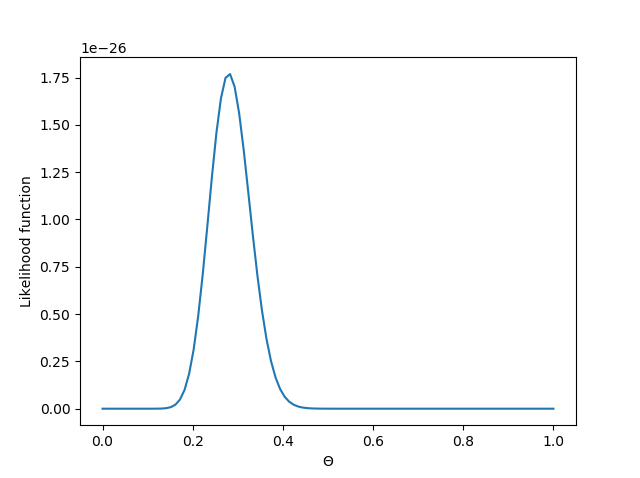
We can see from the plot that \( L \) is maximum at a value close to 0.3. We can differentiate \( L \) to find its maximum. Or we can just use invoke the scipy.optimize function to find the maximum of the likelihood function.
Optimization terminated successfully. Current function value: -0.000000 Iterations: 21 Function evaluations: 42 The likelihood function is maximum at [0.28]
As I mentioned earlier, it is usually easier to minimize the \( log(likelihood) \) function since they have the same \( \theta \) value at which the maximum occurs.
\[ log(L) = p*log(\theta) + (n-p)*log(1-\theta) \]
We will repeat the above process to find the value of \( \theta \) which maximizes \( log(L) \).
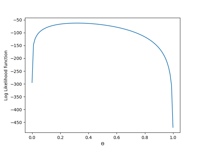
Optimization terminated successfully. Current function value: 59.295332 Iterations: 21 Function evaluations: 42 The likelihood function is maximum at [0.28]
As expected, we find the maximum value at the same value of \( \theta \).
Sampling
Now, because the Bernouilli process that we are using is a random process, the outcomes are different each time. To overcome the possible errors due to randomness, we will sample n values a large number of times (1000). Then using the concept of Central Limit Theorem, we will compute the mean, standard deviation, confidence interval and margin of error in the distribution of \( \theta \).
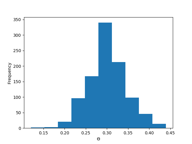
We see a nice normal distribution of the \( \theta \) values resulting from sampling data a bunch of times.
mean of \( \theta \) = 0.2992 Standard error of \( \theta \) = 0.015
95% Confidence interval of \( \theta \) = [0.21 0.38025]
Margin of error
While we already covered mean, standard error and confidence intervals in the last post, the concept of margin of error still requires some attention. Margin of error is another statistic that gives a measure of the random sampling error. Evidently, it has an inverse relationship with the sample size, which is rather intuitive.
Margin of error : \( MOE = z * \frac{\sigma}{\sqrt{n}} \)
where, \( z \) is the z-statistic for the 95% confidence level, and \( \sigma \) is the standard deviation in the sample. Note that \( MOE \propto \frac{1}{\sqrt{n}} \).
Z-score for 95% confidence interval = 1.960 Margin of error=0.009