Dealing with heteroscedasticity in Python
Lately, I have been intrigued by heteroscedasticity, its prevalence in real world datasets and potential means to address the issue. The basic intuition of heteroscedasticity is rather straightforward - consider a distribution which has sub-populations with different variances from the rest. That is, the variance of the residuals is no longer normally distributed. An example is the distribution of income versus education level - the more educated a person is, the more they tend to earn. But the highly educated people also choose to take up philanthropic jobs which tend to pay lesser. This implies that the variance of the distribution is lower at lower education levels and higher at higher education levels.
I found a neat plot that serves as the second example. Note that some of the countries with high average education levels might be socialist and hence not have high per capita income.
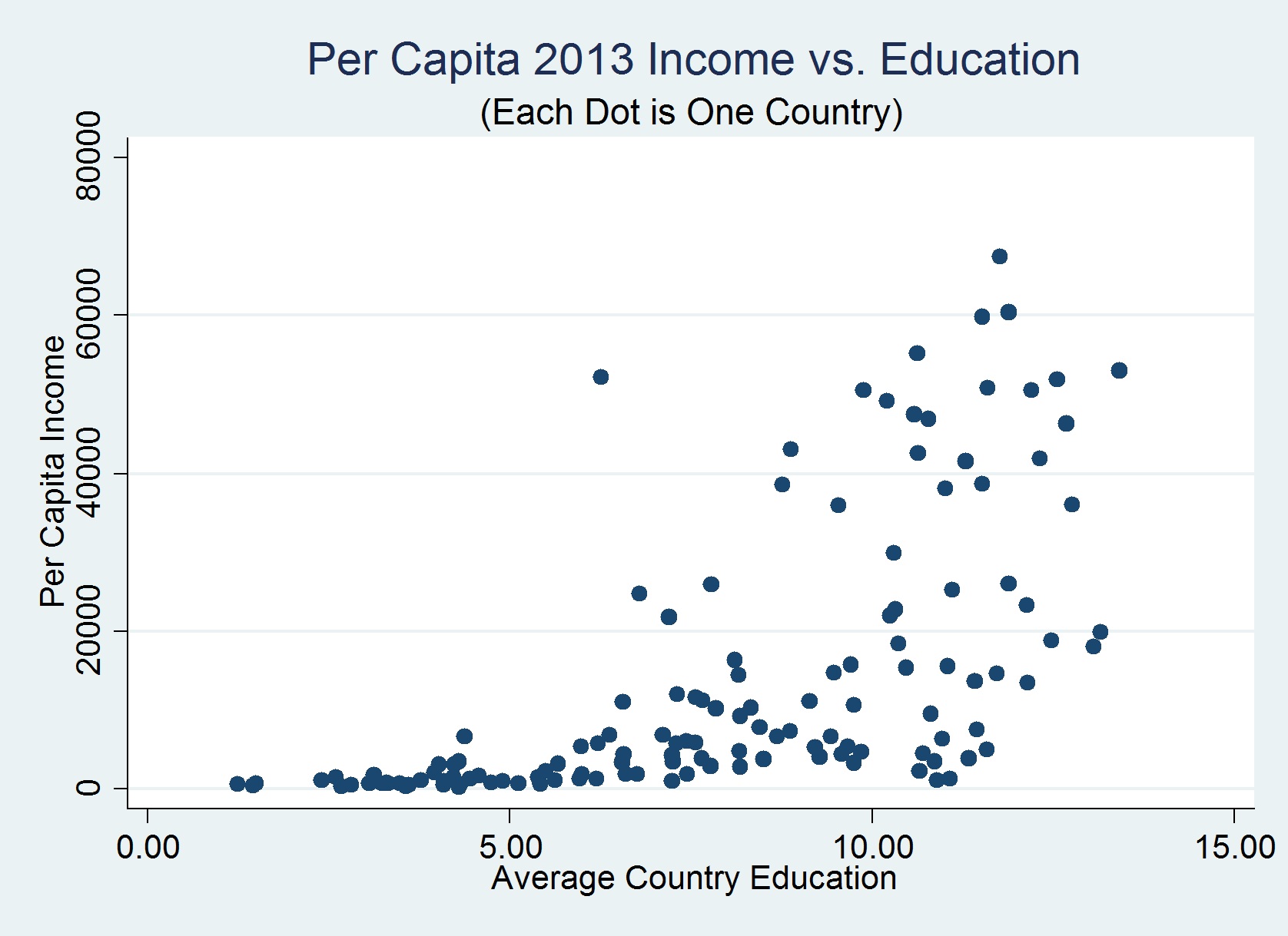
(Image taken from Dr. Naci Mocan’s blog)
Why should we care?
In the above plot, if we fit a typical ordinary least squares (OLS) based linear regression curve (of the form y=ax+b) to the dataset, the fit will be influenced quite severely by the points at higher x values, given the larger variances. This is far from ideal because we do not want the points with large errors to skew the general trend.
What do we do about it?
A standard way to address this issue is to penalize the points at larger variances. If we are seeking a linear fit to the data, the points with the larger noise/errors should be of lower influence than the points that lie close together. Enter weighted least squares (WLS) - in this method, the weights for each datapoint is scaled inversely as a function of its variance, thereby achieving the above goal.
How do we do it?
I have access to some real-world data that exhibits heteroscedasticity. It’s a large dataset of recreation center user swipes (more analysis on this dataset to come in an upcoming post). We will consider just two features - the number of swipes per year and the overall GPA. Note that the below analysis will be performed on a small (randomly sampled) subset of the total dataset (creating hype for my next post). We will simply plot the two features against each other.
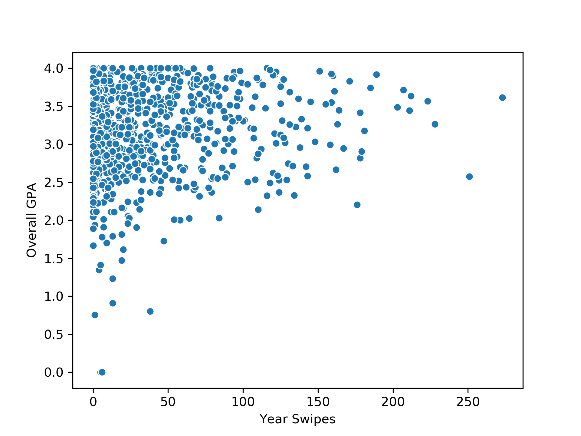
We see that the variance is decreasing with increasing x values. It seems that the students who exercised more had a higher GPA consistently. People who did not exercise had a large distribution of GPAs (the high variance region). We will start with a simple OLS linear regression fit. Some code to follow:
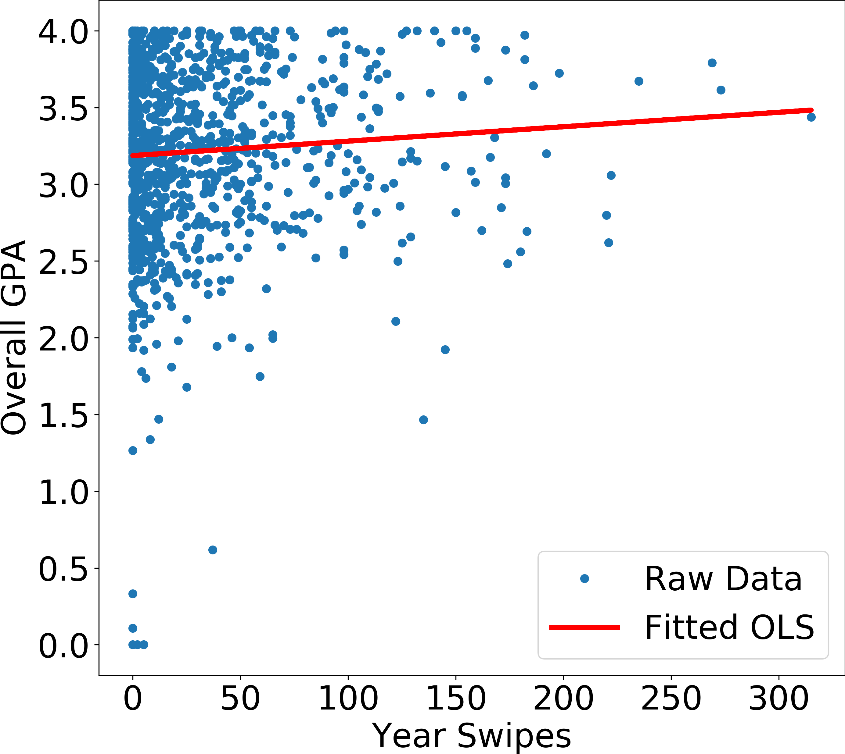
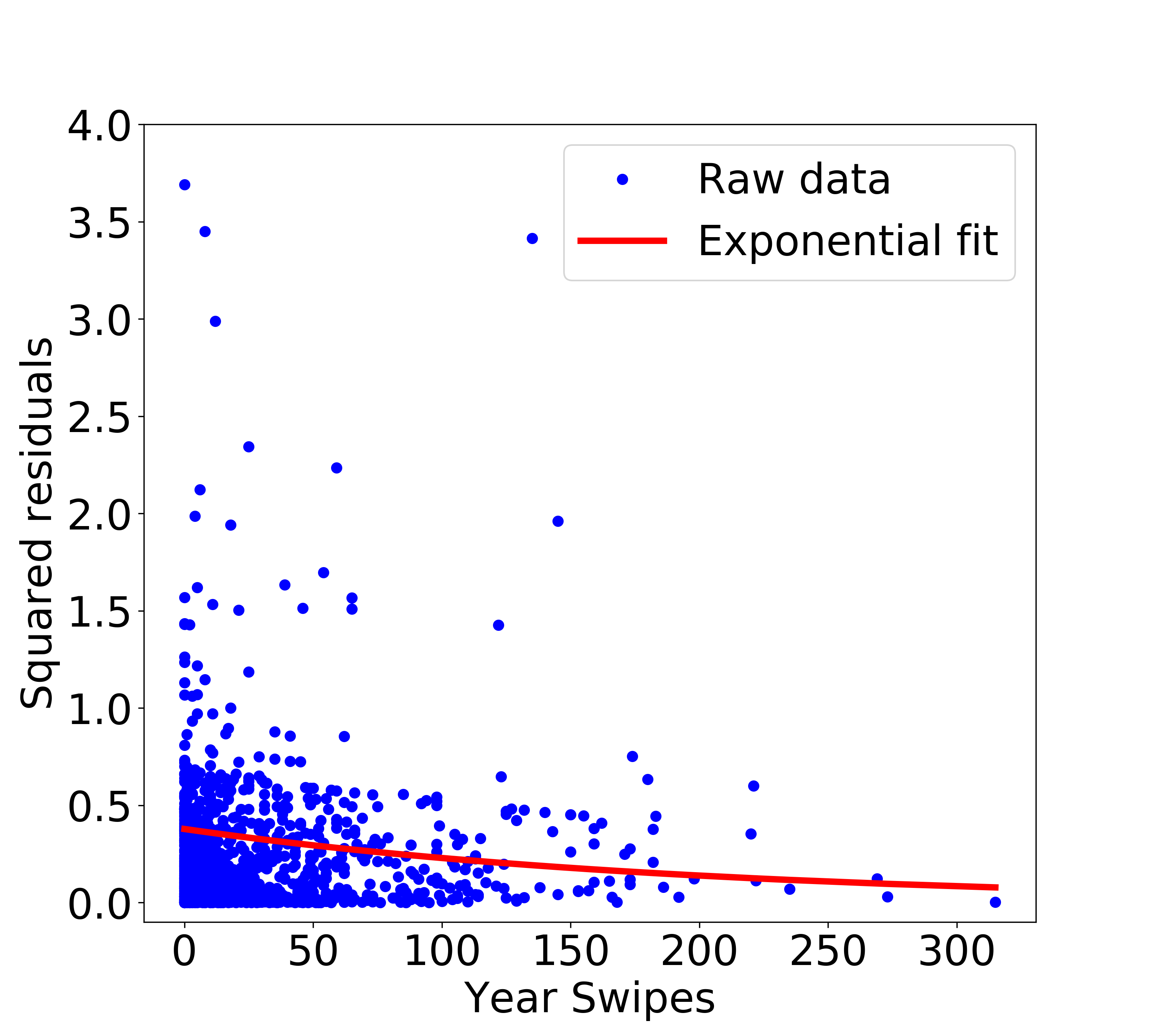
Shown above is an OLS fit to the data. Now, we calculate the squared residuals and plot them as a function of x (Year Swipes). As we can already tell, the squared residuals decreases with increasing x, which is exactly what we find below.
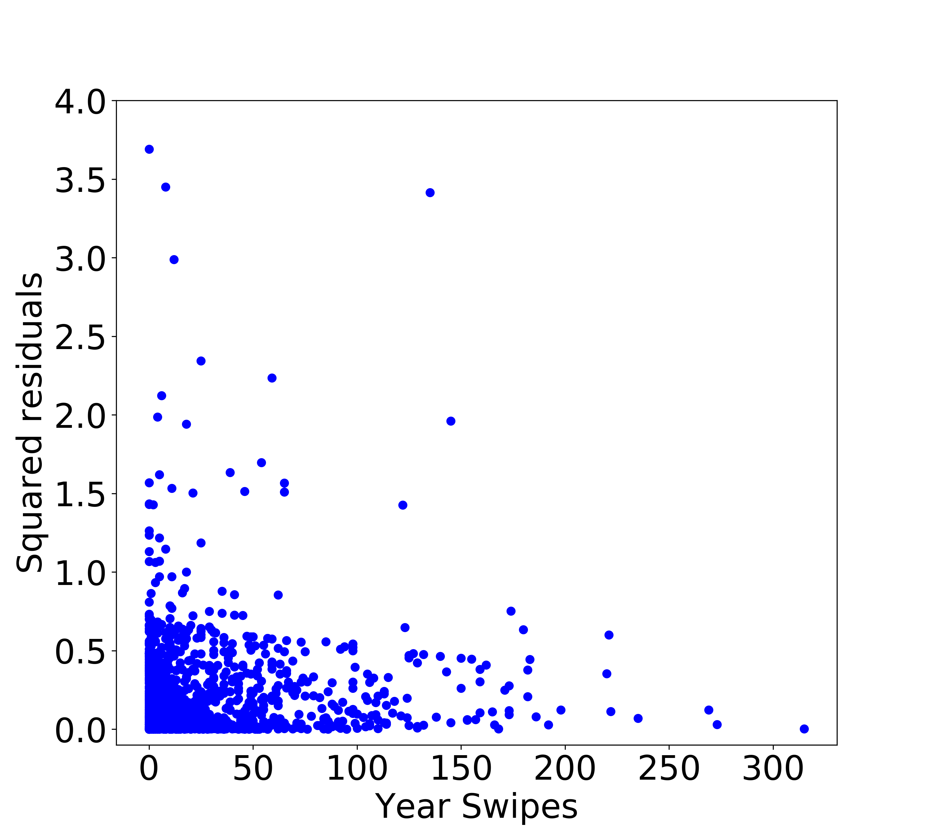
Note that the y axis in the above plot is chopped at 4 to be able to see more detail. Now the important question that we need to answer - how do we use these squared residuals (i.e., variances) to set weights? We know that for WLS, the weights are scaled inversely with the variance, but how exactly do we model variance as a function of the x axis? There are two ways of answering this -
- assuming a parametric form for the dependence of variance with x. From the above plot, my best guess is that the dependence is exponential.
- using a non-parametric algorithm (such as support vector machine) to fit and estimate for every x.
Parametric form
We will assume an exponential form here; scipy to the rescue:
This is certainly a bias we are introducing in the system, but it makes sense to use a parametric form if we have some prior intuition about the form of the variance, i.e., the behavior of the system is known. We will go ahead and use the fitted values to compute the variances, and eventually the weights for WLS. The implementation of WLS in statsmodels is easy:
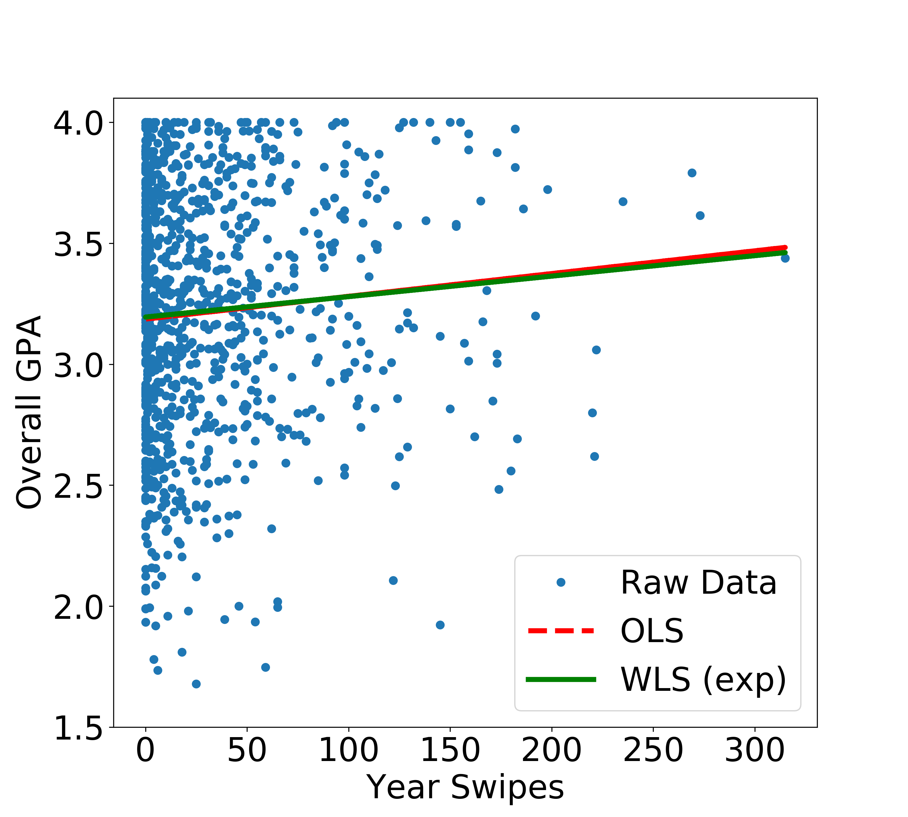
We see that we get a new fitted linear regression line, albeit only slightly different. We will look at evaluating the performance at the end.
Non-parametric form
If we have no idea about the actual form that the variances take or if we just do not want to make such an assumption, we can turn to a non-parametric form such as Support Vector Machine (SVM) or Decision Trees. Here, we will simply use SVM implementation using sklearn. We don’t care much about parameter tuning here since our goal is to roughly model the variance dependence on x.
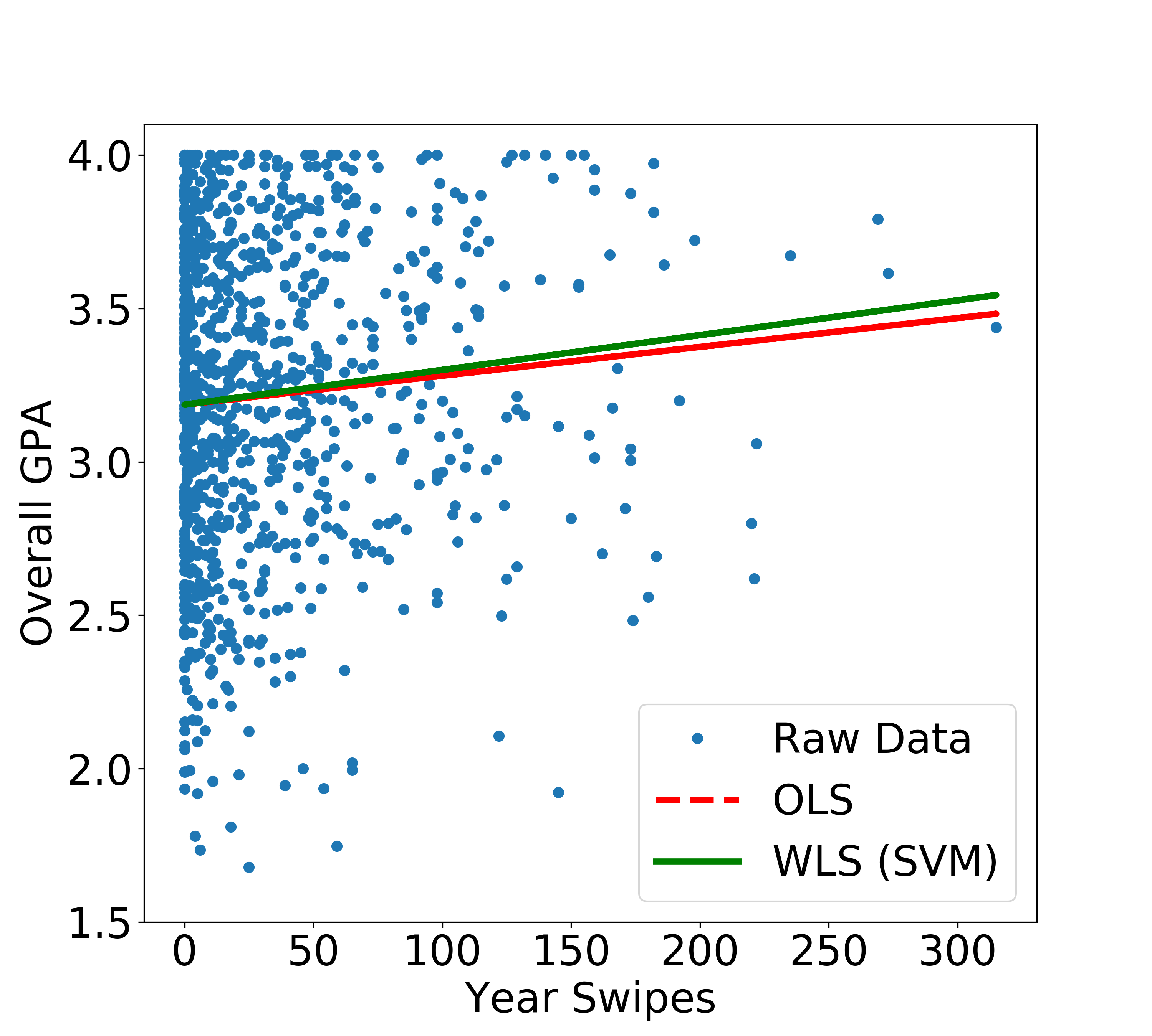
The resulting linear regression curve is quite different from the previous case.
Evaluating performance
We will use standard errors for the two constants a and b (in y=ax+b) as a metric to evaluate the performance of the OLS and the two WLS fits. Evidently, we expect the standard errors for the two constants to decrease when we adopt WLS. The results are summarized below:
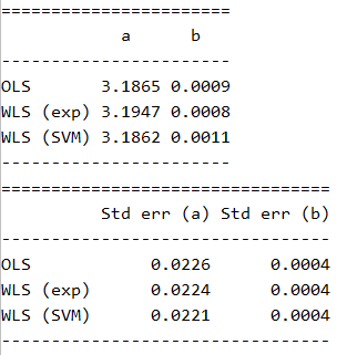
There we go - our standard errors for a decreased in both the cases of WLS. We most certainly have a better fitting linear regression curve by adopting WLS. Although the difference here is minor, in real world applications, a small change in slope could have a significant impact.